Startup and Shutdown Analysis: How to Read Bode and Polar Plots

At steady state, a turbomachine runs at nearly constant speed, so you only get a snapshot of its rotordynamic behavior. During a startup or coastdown, the rotor sweeps its entire speed range and passes through its resonances. That is when the machine reveals where its critical speeds are, how much damping it has, and whether anything has changed since the last transient.

The two classic tools for reading a transient are the Bode plot and the polar plot. This article walks through how to read them, what the amplification factor tells you, why slow roll compensation matters, and how to compare successive startups to catch problems early.

The starting point: the filtered 1X vector

Both plots display the same thing: the filtered 1X vector, the once-per-revolution component of vibration, with its amplitude and phase. To get it, you need:

• Proximity probes in X and Y at each bearing, measuring relative shaft motion in mils pp or µm pp.
• A phase reference (Keyphasor) that produces one pulse per revolution. Phase is the angle between that pulse and the positive peak of the 1X-filtered signal, normally expressed as phase lag.

A tracking filter follows running speed, so every rpm step yields an amplitude/phase pair. That ordered set of vectors is the raw material for everything below. For a refresher on how the X and Y probes combine into shaft motion, see how to interpret shaft orbits.

How to read a Bode plot

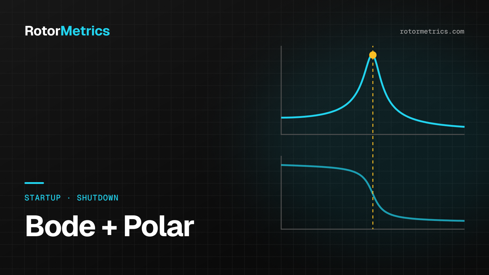
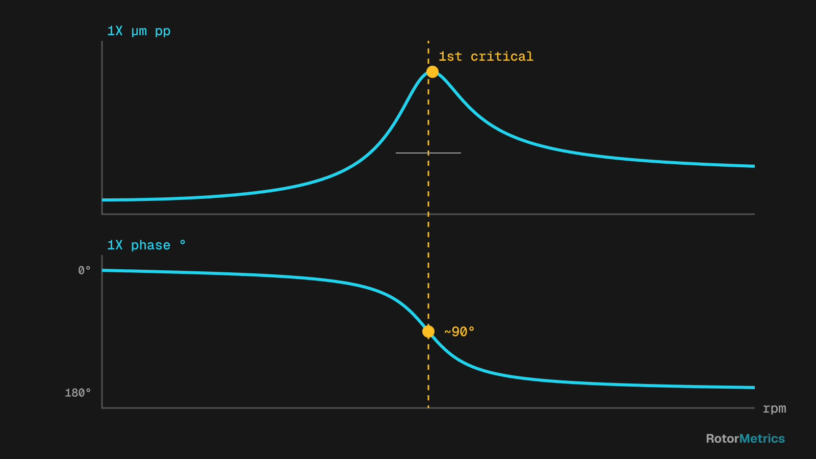
A Bode plot is really two stacked charts that share a horizontal speed axis: 1X amplitude on top and 1X phase lag below.

Identifying a critical speed

A rotor resonance has two signatures that must show up together:

1. An amplitude peak in 1X that rises as speed approaches the critical and falls after passing it.
2. A phase shift over the same speed range. For a simple, well-defined mode, phase lag increases by roughly 90° at the resonance and approaches 180° overall from well below to well above it.

The rule of thumb: a peak without a phase shift is not a rotor resonance. It may be a structural resonance, a process effect, or noise. Conversely, a clear phase shift with only a modest peak usually points to a heavily damped mode.

A few nuances:

• When bearing stiffness differs horizontally and vertically, the X and Y probes may show the critical at slightly different speeds (split criticals). Check both.
• The absolute phase value depends on the instrument and its conventions. What matters is how much it shifts and where.
• Warm-up holds create dense clusters of points on the Bode plot. They are not resonances.

Amplification factor and separation margin

The amplification factor (AF) describes how sharp a resonance is, and therefore how much damping the mode has. API 684 describes the half-power bandwidth method: find the speeds on either side of the peak where amplitude drops to 0.707 of the maximum, then divide the critical speed by the difference between those two speeds. A tall, narrow peak gives a high AF; a broad, gentle peak gives a low one.

The AF drives the separation margin, meaning how far a critical speed must sit from the operating speed range. API 617 and API 684 tie the two together: modes with enough damping (AF below 2.5) are considered critically damped and require no separation margin, while sharper modes do. The exact equations depend on the edition, so check the current standard when qualifying a machine.

In the field, measured AF is most useful for comparison: if the AF of the first critical climbs over time, damping is going down.

How to read a polar plot

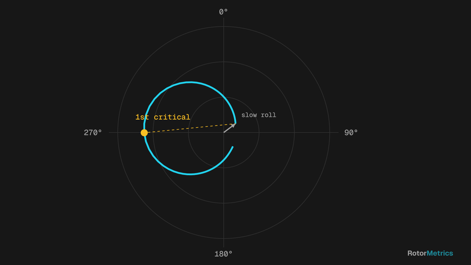
A polar plot shows the same data in polar coordinates. Each point is the tip of the 1X vector, with amplitude as the distance from the center and phase as the angle, connected in speed order.

What to look for:

• A resonance shows up as a loop. The critical speed sits near the point farthest from the origin, about 90° from the low-speed phase.
• Multiple loops mean multiple modes; a distorted loop can expose a structural resonance.
• The curve does not start at the origin. That starting point is the slow roll vector.

The polar plot makes heavily damped modes and, above all, vector changes between transients easy to spot. It is also the natural plot for balancing work, since trial weights are reasoned in vector terms.

Runout (slow roll) compensation

At low speed the rotor has essentially no dynamic response, yet the probe still reads something: mechanical surface imperfections, electrical runout in the shaft material, and any bow. That is the slow roll vector, and it adds to the true response at every speed. To compensate:

1. Pick a low speed with no meaningful dynamic response and stable amplitude and phase.
2. Take the 1X vector at that speed as the reference.
3. Subtract it as a vector (not just in amplitude) from every point on the Bode and polar plots.

After compensation, the polar loop starts at the origin and the Bode plot reflects the true dynamic response. Slow roll is also diagnostic data in its own right: if it changes from one startup to the next, it can indicate a thermal or mechanical bow.

Cascade plots as a complement

Bode and polar plots only see 1X. To see the full spectrum during a transient, use a cascade (waterfall) plot: spectra stacked by speed. It shows order lines (1X, 2X, 3X), fixed-frequency resonances that light up as an order line crosses them, and subsynchronous components typical of oil whirl and oil whip.

For example, a cascade slice where 2X grows abnormally near half the first critical speed deserves a closer look:

Comparing successive startups

A single Bode plot tells you what the machine is like; two overlaid plots tell you what changed. That is why you should save a baseline transient (after an overhaul or a healthy commissioning run) and overlay every new startup or coastdown on it.

Observed change	Possible cause	What to check
Critical speed drops	Loss of stiffness: bearing clearance, loose support, cracked shaft	Clearances, shaft centerline, 2X
Critical rises or peak flattens	Rub adding stiffness at the contact	Orbit shape, harmonics, 1X phase
Higher AF	Less damping	Bearings, oil temperature and pressure
Slow roll vector changes	Thermal or mechanical bow	Prior slow roll time, shutdown history
2X resonance at half the critical	Possible transverse crack	1X and 2X trends

Several of these causes develop slowly, so the trend across multiple transients carries more weight than any single comparison. To place these findings in the bigger picture, see how to detect turbocompressor faults.

What data to capture

• X and Y probes at every bearing plus the phase reference, all synchronized.
• Sampling on speed increments, not just time, so you have enough resolution near the criticals, where things change fast.
• The full slow roll range, at the start of a startup or the end of a coastdown.
• Raw waveforms, not just 1X values, so orbits and cascades can be rebuilt later.
• Context: oil temperature and pressure, load, prior slow roll time, and whether it was a cold or hot start.

Best practices

• Use the coastdown as your reference when possible. It tends to be more repeatable because the rotor decelerates without driver influence.
• Compare like with like: cold start with cold start, hot with hot.
• Always review amplitude and phase together. Many faults show up in phase first.
• Log each transient with the date, the reason for the shutdown, and any work performed.

How RotorMetrics does it

We take the signal from your existing protection system (for example, a Bently Nevada 3500) without modifying it, so every startup and coastdown is recorded with waveforms and phase reference, even when nobody is watching. Our vibration specialists compare each transient against the machine's baseline and let you know if a critical shifted, slow roll changed or something new appears, with a specific recommendation.

Sources

• API RP 684, Rotordynamic Tutorial: Lateral Critical Speeds, Unbalance Response, Stability, Train Torsionals, and Rotor Balancing. American Petroleum Institute.
• API Standard 617, Axial and Centrifugal Compressors and Expander-compressors. American Petroleum Institute.
• Bently, D. E. and Hatch, C. T. Fundamentals of Rotating Machinery Diagnostics. Bently Pressurized Bearing Press, 2002.
• Eisenmann, R. C. Sr. and Eisenmann, R. C. Jr. Machinery Malfunction Diagnosis and Correction. Prentice Hall, 1998.
• Vance, J. M., Zeidan, F. Y. and Murphy, B. Machinery Vibration and Rotordynamics. Wiley, 2010.